One of the many benefits of Bayesian statistics is the ability to incorporate external information in your analysis via a prior. When I last wrote about priors, I described them as your “old belief”. Maybe that’s helpful for an intuitive introduction, but it’s probably better described as prior (or even ‘external’) information.

Priors are the statistical model’s representation of reasonable or plausible values for a parameter (e.g. average/variance of a lognormal distribution). Defining ‘reasonable’ does introduce subjectivity as it requires subject matter expertise. But a defensible prior is one that is based on evidence and also contains the uncertainty that prompted the assessment in the first place. Some scientists may intentionally use less information than they have to satisfy a sceptical audience.

Below I’ll refer to μ (pronounced ‘mew’). It’s the position parameter for a lognormal distribution and is the log of the geometric mean (GM). If you see μ, you can kind of think “GM”.

Types of Priors

One way of thinking about priors is by how much information they provide the model. For once, statistics uses naming conventions that are pretty easy: uninformative, weakly informative, and informative priors. There aren’t strict definitions, but I’ve described these below:

Flat/Uninformative Priors

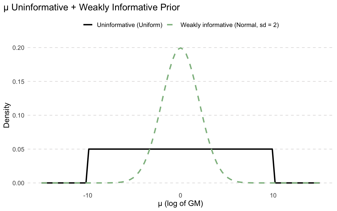
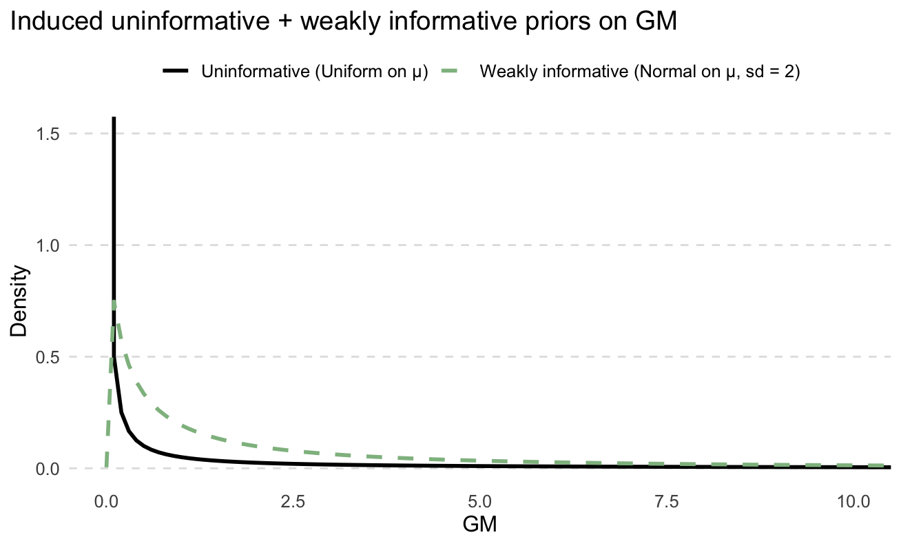
As the name suggests, uninformative priors provide little to no information. They are often uniform or normal distributions that are so wide they basically say that “any value is just as likely as any other value”. Some scientists like it because “it lets the data speak for itself”. A uninformative prior for μ might be uniform(-10, 10). You can interpret this prior as “μ can be any value between -10 to 10, and all values are just as likely”. Remember, μ is on the log scale - this equates to a GM of 0.00005 ppm and 22,000 ppm. Not very precise, huh.

Some authors like Andrew Gelman and Richard McElreath (two great lecturers in statistics, BTW) take issue with these kinds of priors.

You are allowing values for μ (again, think GM) that you know are either extremely unreasonable or downright impossible. You’d hopefully know enough about the exposure scenario to know how to make the range above a bit narrower.
When you have a small dataset as we typically do in hygiene, the confidence/credible intervals can be very wide. Think about the last time you put three respirable dust results into IHstats and got a 95% UCL of 400mg/m³. Flat priors provide nothing to help, and just say, “Hey, maybe the respirable dust average really is 400mg/m³ (probably not!)”
There can be computational issues when using extremely wide priors. The MCMC can get lost or stuck on its walk through the proverbial forest.
A flat prior for μ once converted into the GM is actually not flat at all!

Weakly Informative Priors

Weakly informative priors are designed to not unduly influence or overwhelm the data, only to significantly reduce the chance of those ridiculous values from uninformative priors. Perhaps a prior for μ of normal(log(0.5), 2²). This would mean that we are approximately 95% sure the GM is between 0.01 and 25 ppm, centred around 0.5 ppm. This is still pretty wide but stops those crazy UCL values. Whether or not this is appropriate depends on the situation. Arguably the exact values used can be somewhat arbitrary but at the very least they are explicit so we can have that argument in the first place. At large enough sample sizes, the data will overwhelm the informative provided by the weak prior and the exact values won’t matter.

Also, perhaps the priors shown below look rather informative but they have deceptively wide tail. Again, what’s appropriate will change between situations.

Informative Priors

Informative priors are where the real magic (and controversy) comes in. You’re bringing in a lot of information to help supplement that data you collect. At large sample sizes, the data may still overwhelm the prior, but it’s at small sample sizes that informative priors can have a significant impact on the outcomes and the resulting decisions. This is why informative priors can be controversial and usually require a strong justification. Professional judgement is usually not enough to convince a sceptical audience. Typically, you would want to use historical data or modelling or data from literature. Harrison Quick et al. (2017) wrote about using the normal-inverse gamma distributions to create informative priors. This uses historical data but applies a weighting to control the uncertainty or the information provided by those priors. The more historical data, the more informative the prior (to a certain point).

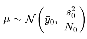
The μ prior used in Quick (2017). *yˉ0 = sample mean of logged historical data, s²_0 is variance of logged historical data, and N_0 is the effective sample size of the historical data*

Notice the N₀. This is the number of samples in the historical data. More samples result in a lower variance of μ and therefore more precision/certainty as to the value of μ. But you can control this value yourself, effectively dialling up or down the amount of information. In the paper, they recommend limiting N₀ not to be less than the sample size of the new data, and a hard upper limit of 5, so that no matter how much historical data you have, it will not be completely overwhelmed by the prior. You can still have more than 5 historical samples, but the effective sample size (N₀) is capped.

Conjugate Priors

Normally, Bayesian analysis is so complex that it can’t be solved directly. It requires the use of an MCMC that solves the posterior (the results) piece by piece instead of all at once.

However, when the prior and posterior are of the same family, it can work out that they can be solved algebraically. There’s a ‘closed form’ that can be calculated without the use of an MCMC. When the prior and posterior match like this, they are called conjugate. Back in the day, conjugate priors were very convenient (and practically essential) as MCMCs are computationally intense. But with modern-day computing, it is no longer necessary (though still sometimes useful). You can now essentially use whichever distribution suits your needs best.

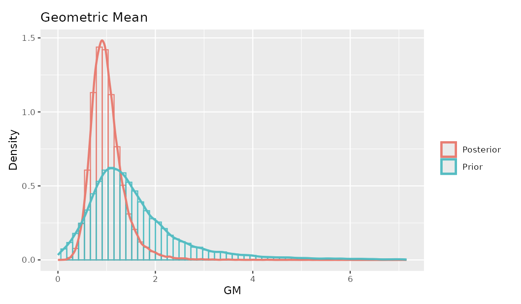
Tool

I have created a tool that mimics the model presented in the Quick paper that was mentioned previously. It shows you the priors created from historical data that you put in and the posterior (the results of the statistical analysis). Have a play and see how different data and different amounts of data create different priors and posteriors.

That tool differs from the approach in Quick et al. in two ways. First, their paper fits the model using MCMC, whereas the tool solves algebraically (they used conjugate priors!). Second, and more subtly, Quick et al. treat the prior variance hyperparameter s² as fixed when constructing the prior for μ, rather than tying it hierarchically to the uncertainty in σ² as is common in fully hierarchical models described by Gelman. This might be to keep things a bit more simple.

Questions

Some questions I’ve been asked about priors:

If I have historical data from the SEG, why would I just group them together in the analysis? What difference does it make?

You certainly could bundle historical data rather than creating an informative prior. Whether this is valid would depend on how old the data is and whether it’s representative of current conditions. If you think the data is still useful but not sure if conditions are exactly the same, this uncertainty can be incorporated into the prior. Whether it makes a difference depends on how much data you have in each set and how you set up the model.

Couldn’t someone use informative priors to manipulate the results to get the answer they want?

Yes. That’s partly why it’s important as an author to be transparent, and why as a reader to be sceptical.

What would a regulator or court think?

I’m not sure. I’m not aware of a case relating to occupational exposures in which the choice of statistical model played a role in evidence. I would guess that if you used sound statistical principles and clearly articulated reasoning, it would be defensible. Again: think of the sceptical audience.

Reference

Quick, H., Huynh, T., & Ramachandran, G. (2017). A Method for Constructing Informative Priors for Bayesian Modeling of Occupational Hygiene Data. Annals of Work Exposures and Health, 61(1), 67-75. https://doi.org/10.1093/annweh/wxw001

A.I. was used to proofread this blog and the code for the tool. The content was written entirely by me with regard to the materials referenced.

What’s a Prior?